library(tidyverse)5 Bayesian inference in discrete case
Date: 2026-01-31
6 Load libraries
7 Bayesian inference in discrete case: simple example
The scenario (taken from Dr. Jingchen (Monika) Hu from youtube, S22 Math 347 course): A chinese food restaurant owner wants to increase the business profits and wants to know when people prefer to come into her restaurant. Specifically, she is interested in how often people chose Friday. So, Friday = “success”, and all other days are considered “failures”. She wants to use a Bayesian approach to estimate the probability that patrons will believe Friday is their favorite day to eat.
7.1 Steps
She wants to use a Bayesian approach and involves the following steps:
Set up the prior expectations of success \(\pi(p)\) or \(\pi(success)\)
Collect data and estimate the likelihood -> use binomial distribution
Likelihood of p and Binomial probability mass function (pmf):\[\pi(y|p_{i})=L(p_{i})=P(Y = y) = \binom{n}{y} p^y (1-p)^{n-y}\]
Assumptions of binomial experiment:
- repeating same task/trial many times
- on each trial, 2 possible outcomes: “success” or “failure”
- Prob of success, p, same for each trial
- Results of outcomes from different trials are independent
- Apply Baye’s rule
Bayes rule: \[\pi(p_{i}| y) = \frac{\pi(y|p_{i}) \times \pi(p_{i})}{\pi(y)} \]
\[\pi(y) = \sum_{j} \pi(p_{j}\times L(p_{j})) \]
The denominator gives the marginal distribution of the observation \(y\) by the law of total probability.
7.2 Set up prior \(\pi(p)\)
#probabilities of success to consider
p<-seq(.3,.8,.1)
#p

#probabilities for each of p
prior<-c(.125,.125,.25,.25,.125,.125)

d<-tibble(prior,p)

ggplot(d,aes(x=p,y=prior))+geom_bar(stat="identity")+theme_bw()+scale_x_continuous(limits=c(0,1),breaks=seq(0,1,.1),labels=seq(0,1,.1))+ylab("prior probability")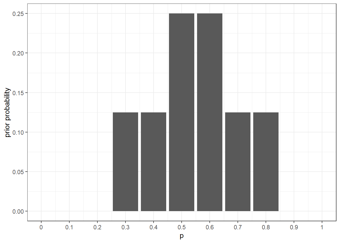
7.3 Calculate likelihood -binomial
She surveyed 20 patrons and 12 chose Friday. So this looks like
\[L(p_{i}) = \binom{20}{12}p^{12}\times (1-p)^{20-12}\]
#use the density binomial function , dbinom()
d$likelihood<-dbinom(x=12,size=20,prob=d$p)
knitr::kable(d)| prior | p | likelihood |
|---|---|---|
| 0.125 | 0.3 | 0.0038593 |
| 0.125 | 0.4 | 0.0354974 |
| 0.250 | 0.5 | 0.1201344 |
| 0.250 | 0.6 | 0.1797058 |
| 0.125 | 0.7 | 0.1143967 |
| 0.125 | 0.8 | 0.0221609 |
7.4 Apply Baye’s rule and calculate the posterior probability (\(\pi(p_{i}|y)\))
\(\pi(p_{i}|y)\) is the posterior probability of \(p = p_{i}\) given the number of successes \(y\).
d$marg<-sum(d$prior*d$likelihood)

d$posterior<-(d$prior*d$likelihood)/d$marg

#plot table
knitr::kable(d)| prior | p | likelihood | marg | posterior |
|---|---|---|---|---|
| 0.125 | 0.3 | 0.0038593 | 0.0969493 | 0.0049759 |
| 0.125 | 0.4 | 0.0354974 | 0.0969493 | 0.0457680 |
| 0.250 | 0.5 | 0.1201344 | 0.0969493 | 0.3097865 |
| 0.250 | 0.6 | 0.1797058 | 0.0969493 | 0.4634013 |
| 0.125 | 0.7 | 0.1143967 | 0.0969493 | 0.1474955 |
| 0.125 | 0.8 | 0.0221609 | 0.0969493 | 0.0285728 |
#let's plot everything out
#ggplot(d,aes(x=p,y=posterior))+geom_point()
7.4.1 inferential question: What is the posterior prob that over half of the customers prefer to eat out on friday for dinner?
an<-d|>
  filter(p>.5)|>
  dplyr::summarise(oh=sum(posterior))
\(Prob(p>0.5) =\) 0.6394696
7.4.2 Let’s plot out the prior, likelihood, and posterior
I’m going to normalize the likelihood function with 3x the max for plottig purposes.
d$sl<-d$likelihood/(max(d$likelihood)*3)

d2<-d|>
  select(p,prior,sl,posterior)|>
  pivot_longer(prior:posterior)|>
  mutate(parameter=if_else(name=="prior","Prior",if_else(name=="sl","Likelihood","Posterior")))


ggplot(d2,aes(x=p,y=value,colour=parameter))+geom_point()+geom_line(linewidth=1)+xlab("Probability")+ylab("Density")+theme_bw()+theme(legend.position="top")+scale_colour_manual(name="",values=c('#AA1E2D','#46A6B2','#18272F'))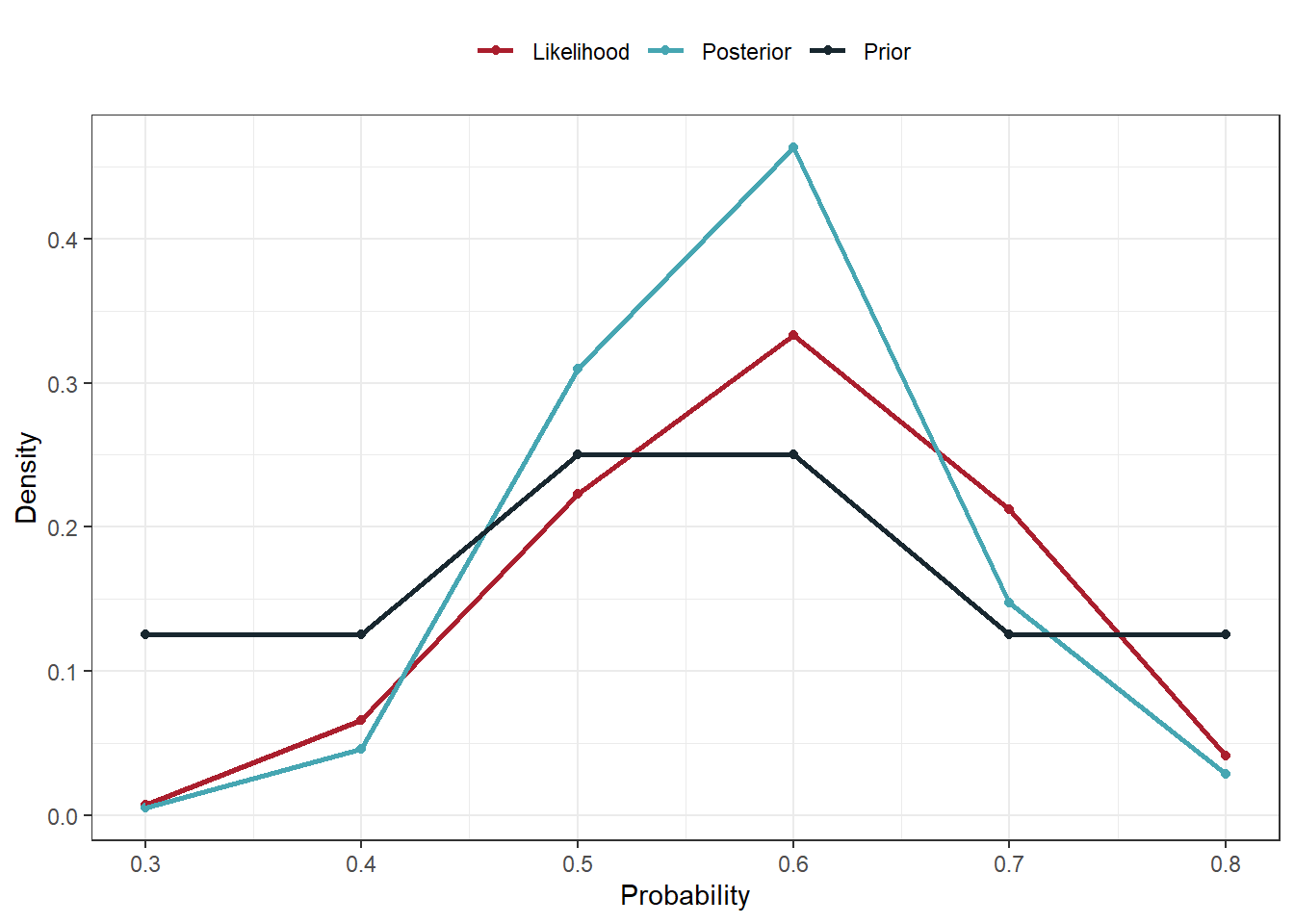
8 Sessioninfo
sessionInfo()R version 4.5.0 (2025-04-11 ucrt)
Platform: x86_64-w64-mingw32/x64
Running under: Windows 11 x64 (build 26100)
Matrix products: default
LAPACK version 3.12.1
locale:
[1] LC_COLLATE=English_United States.utf8
[2] LC_CTYPE=English_United States.utf8
[3] LC_MONETARY=English_United States.utf8
[4] LC_NUMERIC=C
[5] LC_TIME=English_United States.utf8
time zone: America/New_York
tzcode source: internal
attached base packages:
[1] stats graphics grDevices utils datasets methods base
other attached packages:
[1] lubridate_1.9.4 forcats_1.0.0 stringr_1.5.1 dplyr_1.1.4
[5] purrr_1.0.4 readr_2.1.5 tidyr_1.3.1 tibble_3.2.1
[9] ggplot2_3.5.2 tidyverse_2.0.0
loaded via a namespace (and not attached):
[1] gtable_0.3.6 jsonlite_2.0.0 compiler_4.5.0 tidyselect_1.2.1
[5] scales_1.3.0 yaml_2.3.10 fastmap_1.2.0 R6_2.6.1
[9] labeling_0.4.3 generics_0.1.3 knitr_1.50 htmlwidgets_1.6.4
[13] munsell_0.5.1 pillar_1.10.2 tzdb_0.5.0 rlang_1.1.6
[17] stringi_1.8.7 xfun_0.52 timechange_0.3.0 cli_3.6.4
[21] withr_3.0.2 magrittr_2.0.3 digest_0.6.37 grid_4.5.0
[25] hms_1.1.3 lifecycle_1.0.4 vctrs_0.6.5 evaluate_1.0.3
[29] glue_1.8.0 farver_2.1.2 colorspace_2.1-1 rmarkdown_2.29
[33] tools_4.5.0 pkgconfig_2.0.3 htmltools_0.5.8.1