library(tidyverse)
library(gt)7 Bayesian sequential analysis
8 Load library
9 Introduction
In this script, I’m simulating sequential patient monitoring in a single-arm clinical trial. Here are the conditions that we can modify in the simulation:
- Number of simulations
- True event probability and target probability for decision making
- Prior: \(\beta(1,1)\), which is a flat prior
- Total sample size
- Sequential monitoring start at a given sample size
- Sequential monitoring step (every 1 patient is default)
- Posterior after n patients is: $p|data (1+x, 1+n-x) $
At each look, evaluate:
- Futility threshold
- Early efficacy threshold
- Otherwise continue
10 Simulation set up
# Bayesian beta-binomial 1-arm simulation with configurable thresholds
# Includes posterior bias = (posterior mean at stopping - true probability)
simulate_trial <- function(true_p = 0.30,
                           target_p = 0.30,
                           maxN = 200,
                           start_monitor = 50,
                           monitor_every = 1,
                           prior_a = 1,
                           prior_b = 1,
                           futility_threshold = 0.05,   # stop if Pr(p > target_p) < futility_threshold
                           efficacy_threshold = 0.50,   # stop if Pr(p > target_p) >= efficacy_threshold
                           nsim = 1,
                           return_both = c("data", "summary")) {
  stopifnot(start_monitor >= 1, maxN >= start_monitor,
            monitor_every >= 1, nsim >= 1)
  return_both <- match.arg(return_both)

  # Storage for per-simulation results
  results <- data.frame(
    sim = integer(nsim),
    n = integer(nsim),
    x = integer(nsim),
    decision = character(nsim),
    post_mean = numeric(nsim),
    post_lcl = numeric(nsim),
    post_ucl = numeric(nsim),
    pr_gt_p = numeric(nsim),
    posterior_bias = numeric(nsim),   # NEW: posterior mean - true_p
    stringsAsFactors = FALSE
  )

  for (s in seq_len(nsim)) {
    # Generate Bernoulli outcomes under the true event rate
    outcomes <- rbinom(maxN, size = 1, prob = true_p)

    decision <- "Max Sample"
    n_final <- maxN
    x_final <- sum(outcomes)

    looks <- seq(from = start_monitor, to = maxN, by = monitor_every)

    for (n in looks) {
      x <- sum(outcomes[1:n])

      # Posterior parameters for Beta(prior_a, prior_b)
      post_a <- prior_a + x
      post_b <- prior_b + (n - x)

      # Analytic posterior probability Pr(p > target_p)
      pr_gt <- 1 - pbeta(target_p, shape1 = post_a, shape2 = post_b)

      # Futility rule
      if (pr_gt < futility_threshold) {
        decision <- "Futility"
        n_final <- n
        x_final <- x
        break
      }

      # Early efficacy rule
      if (pr_gt >= efficacy_threshold) {
        decision <- "Early Efficacy"
        n_final <- n
        x_final <- x
        break
      }
      # Else continue
    }

    # Posterior summaries at stopping point (or maxN)
    post_a <- prior_a + x_final
    post_b <- prior_b + (n_final - x_final)

    post_mean <- post_a / (post_a + post_b)
    post_ci <- qbeta(c(0.025, 0.975), shape1 = post_a, shape2 = post_b)
    pr_gt_p <- 1 - pbeta(target_p, shape1 = post_a, shape2 = post_b)
    posterior_bias <- post_mean - true_p   # NEW

    # Save results
    results$sim[s]            <- s
    results$n[s]              <- n_final
    results$x[s]              <- x_final
    results$decision[s]       <- decision
    results$post_mean[s]      <- post_mean
    results$post_lcl[s]       <- post_ci[1]
    results$post_ucl[s]       <- post_ci[2]
    results$pr_gt_p[s]        <- pr_gt_p
    results$posterior_bias[s] <- posterior_bias
  }

  # Summaries across simulations
  decision_table <- table(results$decision)
  ess <- mean(results$n)
  mean_post_mean <- mean(results$post_mean)
  mean_posterior_bias <- mean(results$posterior_bias)  # NEW (same as mean_post_mean - true_p)

  summary <- list(
    settings = list(
      true_p = true_p,
      target_p = target_p,
      maxN = maxN,
      start_monitor = start_monitor,
      monitor_every = monitor_every,
      prior_a = prior_a,
      prior_b = prior_b,
      futility_threshold = futility_threshold,
      efficacy_threshold = efficacy_threshold,
      nsim = nsim
    ),
    decisions = decision_table,
    expected_sample_size = ess,
    mean_post_mean = mean_post_mean,
    mean_posterior_bias = mean_posterior_bias
  )

  if (return_both == "data") {
    return(results)
  } else if (return_both == "summary") {
    return(list(results = results, summary = summary))
  }
}
11 Running simulation
The target and true probability is 0.1 and I want to do 10,000 simulations.Max sample size is 200.
trialsim1<-simulate_trial(true_p = 0.1,target_p=.1,nsim=10000)

#count decisions
results<-trialsim1|>
  dplyr::count(decision)|>
  dplyr::mutate(proportion=round(n/sum(n),3))
results|>
gt()| decision | n | proportion |
|---|---|---|
| Early Efficacy | 8258 | 0.826 |
| Futility | 1261 | 0.126 |
| Max Sample | 481 | 0.048 |
#For the ones that go to max sample, did we reach the goal?
goalmax<-trialsim1|>
  filter(decision=="Max Sample")|>
  dplyr::mutate(goal=if_else(pr_gt_p>=.5,1,0))
mean(goalmax$goal)
[1] 0#none of the max sample sizes reached their goal For this simulation, it looks like futility is too stringent. Let’s try reducing futility threshold and increasing sample size
- Max sample size = 500
- Threshold for futility = 0.025
trialsim2<-simulate_trial(true_p = 0.1,target_p=.1,nsim=10000,maxN = 500,futility_threshold = 0.025)

trialsim2|>
  dplyr::count(decision)|>
  dplyr::mutate(percent=n/sum(n))
decision n percent
1 Early Efficacy 8825 0.8825
2 Futility 883 0.0883
3 Max Sample 292 0.0292#these look like better operating characteristics
#For the ones that go to max sample, did we reach the goal?
goalmax2<-trialsim2|>
filter(decision=="Max Sample")|>
dplyr::mutate(goal=if_else(pr_gt_p>=.5,1,0))
mean(goalmax2$goal)[1] 0#no
#Let's calculate the average sample size for early efficacy
trialsim2|>
filter(decision=="Early Efficacy")|>
summarize(meann=mean(n)) meann
1 71.6834#~71 patients
#Let's see how biased we are for early stopping
trialsim2|>
filter(decision=="Early Efficacy")|>
ggplot(aes(x=post_mean))+geom_histogram()+scale_x_continuous(limits=c(0,.4),breaks=seq(0,.4,.025),labels=seq(0,.4,.025))`stat_bin()` using `bins = 30`. Pick better value with `binwidth`.Warning: Removed 2 rows containing missing values or values outside the scale range
(`geom_bar()`).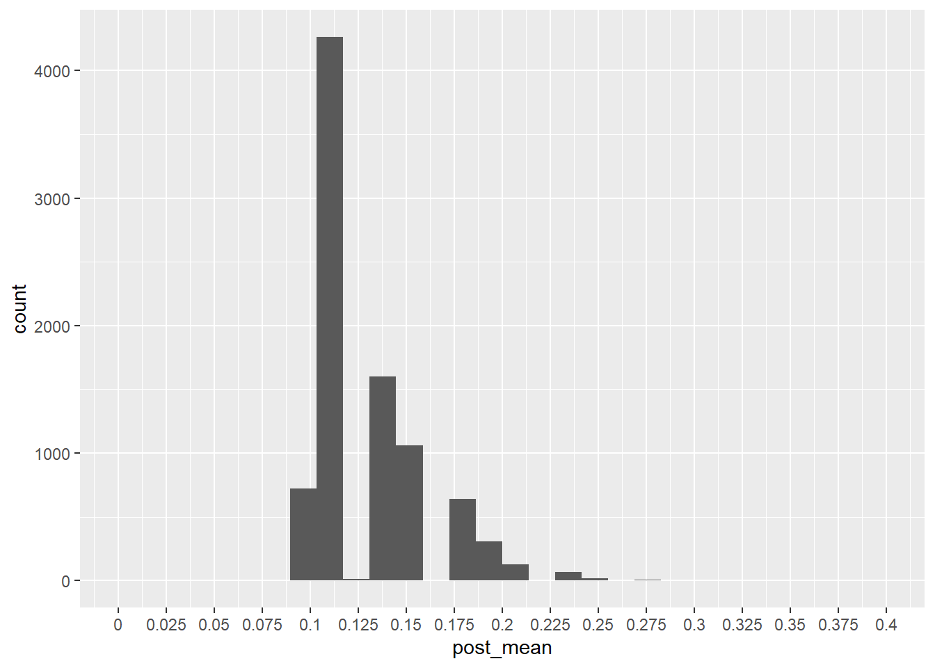
#Let's see how many are within acceptable level of bias , say 0.8-.15?
trialsim2|>
  filter(decision=="Early Efficacy")|>
  dplyr::mutate(accept=if_else(post_mean>=0.8 | post_mean<=0.15,1,0))|>
  summarize(`Acceptable bias`=mean(accept),`Not acceptable bias`=1-`Acceptable bias`)|>
  round(2)
Acceptable bias Not acceptable bias
1 0.75 0.2512 Ways to limit early futility
Lower futility threshold
trialsim3<-simulate_trial(true_p = 0.1,target_p=.1,nsim=10000,maxN = 1000,futility_threshold = 0.01,start_monitor = 100)

#trial results
trialsim3|>
  dplyr::count(decision)|>
  dplyr::mutate(percent=n/sum(n))
decision n percent
1 Early Efficacy 8934 0.8934
2 Futility 516 0.0516
3 Max Sample 550 0.055013 Concluding remarks
This simulation code lets you simulate different scenarios for one-arm studies. You can change the true probability, target probability, number of simulations, sample sizes, thresholding, and when you want to start monitoring.
14 Session info
sessionInfo()R version 4.5.0 (2025-04-11 ucrt)
Platform: x86_64-w64-mingw32/x64
Running under: Windows 11 x64 (build 26100)
Matrix products: default
LAPACK version 3.12.1
locale:
[1] LC_COLLATE=English_United States.utf8
[2] LC_CTYPE=English_United States.utf8
[3] LC_MONETARY=English_United States.utf8
[4] LC_NUMERIC=C
[5] LC_TIME=English_United States.utf8
time zone: America/New_York
tzcode source: internal
attached base packages:
[1] stats graphics grDevices utils datasets methods base
other attached packages:
[1] gt_1.0.0 lubridate_1.9.4 forcats_1.0.0 stringr_1.5.1
[5] dplyr_1.1.4 purrr_1.0.4 readr_2.1.5 tidyr_1.3.1
[9] tibble_3.2.1 ggplot2_3.5.2 tidyverse_2.0.0
loaded via a namespace (and not attached):
[1] gtable_0.3.6 jsonlite_2.0.0 compiler_4.5.0 tidyselect_1.2.1
[5] xml2_1.3.8 scales_1.3.0 yaml_2.3.10 fastmap_1.2.0
[9] R6_2.6.1 labeling_0.4.3 generics_0.1.3 knitr_1.50
[13] htmlwidgets_1.6.4 munsell_0.5.1 pillar_1.10.2 tzdb_0.5.0
[17] rlang_1.1.6 stringi_1.8.7 xfun_0.52 sass_0.4.10
[21] timechange_0.3.0 cli_3.6.4 withr_3.0.2 magrittr_2.0.3
[25] digest_0.6.37 grid_4.5.0 hms_1.1.3 lifecycle_1.0.4
[29] vctrs_0.6.5 evaluate_1.0.3 glue_1.8.0 farver_2.1.2
[33] colorspace_2.1-1 rmarkdown_2.29 tools_4.5.0 pkgconfig_2.0.3
[37] htmltools_0.5.8.1