library(tidyverse) #data parsing and visualization
library(gtsummary) #this lets you create nice tables
library(gt) # create nice tables
library(brms) # bayesian modeling
#library(REDCapDM) # interacting with redcap API
library(splines)
library(marginaleffects)
#library(survival)
library(ggbeeswarm)
library(patchwork)
library(tidybayes)


brms_summary <- function(x) {
  posterior::summarise_draws(x, "mean", "sd",  ~quantile(.x, probs = c(.025,0.975)))
}12 Ordinal regression modeling
13 Load libraries
14 Introduction
In this script, I’m going to simulate different ordinal outcomes to explore how the ordinal regression modelling works. Some ideas to explore-
- Simply analyzing a continuous outcome as ordinal - Frank Harrell says there is a lot of power by doing this.
- 5 ordinal scale - 1-4 is qol and 5 is death
- Get outcomes in terms of probability 1, <2, <4, 5
- Simulate proportional odds and non-proportional odds: evaluate models
- Explore longitudinal aspect
14.1 Notes on ordinal regression models
Taking notes from ordinal regression in brms github.
Ordinal data are categories that show grades of an outcome. Ordinal regression models (cumulative models) assumes that the ordinal variable comes from a categorization of a latent (not observed) continuous \(\hat{Y}\) variable.
Example of ordinal data:
knitr::kable(tibble(groups=c("fundamentalist","moderate","liberal"),`1`=c(40,25,23),`2`=c(54,41,31),`3`=c(119,135,113),`4`=c(55,71,122)))| groups | 1 | 2 | 3 | 4 |
|---|---|---|---|---|
| fundamentalist | 40 | 54 | 119 | 55 |
| moderate | 25 | 41 | 135 | 71 |
| liberal | 23 | 31 | 113 | 122 |
Assuming 4 categories:
There are \(K\) thresholds \(\tau_k\) which partition \(\hat{Y}\) into K+1 observable, ordered categories of \(Y\). With 4 categories assumed, there are K+1=4 response categories, and K=3 thresholds.
Assuming \(\hat{Y}\) follows a normal distribution with a cumulative distribution function \(F\) (CDF), then the probability of \(Y\) being equal to category \(k\) is:
\[Pr(Y=k)= F(\tau_k)-F(\tau_{k-1})\] The CDF of a threshold is subtracted from the CDF of the next lower level threshold to obtain the probability of Y being in a certain category.
Example: \(\phi\) is a normal CDF
\[Pr(Y=2)=\phi(\tau_2) - \phi(\tau_1) = \phi(1)-\phi(-1)= 0.84 -0.16 = 0.68\]
We need to incorporate and describe a regression model. So, the linear regression for \(\hat{Y}\) with predictors is \(\eta=b_1x_1+b_2x_2+..,\), so that \(\hat{Y}= \eta + \epsilon\), where \(\epsilon\) is the error term in the regression. Then, \(\hat{Y}\) can be split into these two parts. Note that there is no intercept in the predictor term because the thresholds \(\tau_k\) replace the model’s intercept as both are not identified at the same time. Thus, the probabilities of \(Y\) being equal to category \(k\) given the linear predictor \(\eta\) is:
\[Pr(Y=k|\eta)= F(\tau_k-\eta) - F(\tau_{k-1}-\eta)\]
Thus..
\[\hat{Y} = \eta + \epsilon = b_1 x_1 + b_2 x_2 + \epsilon\] Assuming the latent variable \(\hat{Y}\) is normally distributed, then the probabilities for each response cateogry \(k\) can be computed as:
\[Pr(Y=k) = \phi(\tau_k-(b_1x_1 + b_2x_2))-\phi(\tau_{k-1}-(b_1x_1 + b_2 x_2))\]
There are also other models: sequential model (where movement across ordinal values depends on the last ordinal value), and the adjacent category model. Appendix A has more details.
14.1.1 Practical application notes
- We can specify a few different models, all of which can be compared with leave-one-out cross validation (LOO).
- If comparing ACM, CM, and SM models, especially with category specific effects (\(cs()\)), then LOO should be also compared with model not specified with \(cs()\).
- If comparing ACM, CM, and SM models, especially with category specific effects (\(cs()\)), then LOO should be also compared with model not specified with \(cs()\).
- brms can explore and account for unequal variances that can vary with predictors (but not cut off values).
- brms can specify different levels of effects across different response categories. This is specified by \(cs()\) function. Category specific estimates are not problematic for SM and ACM models, but there could be negative probabilities for cumulative models.
- Rhat and ESS are checked for chain convergence. Rhat should not be above 1.1 and ESS should be as high as possible. ESS >1000 is a rule of thumb for stable estimates.
15 Let’s first simulate a dataset for proportional ordinal regression
#Let's set up probabilities, then add in some simulate outcomes based on those probabilities
ss<-1000 # sample size
control.prob<-c(0.1,.2,.3,.25,.15)
#sum(control.prob)# has to add up to 1
OR<-.5 # odds ratio

#creat cdf for treatment which is a function of control cdf that has an OR applied to it
t.prob<-plogis(qlogis(cumsum(control.prob)[1:4]) - log(OR))
#from cdf, back calculate to probabilities
t.prob1<-tibble(prob=c(t.prob[1],diff(t.prob),1-t.prob[4]))

#sample data ; control and treatment
#control
control<-sample(size=ss,x=1:5,prob=control.prob,replace=TRUE)
#treatment
trt<-sample(size=ss,x=1:5,prob=t.prob1$prob,replace=TRUE)

#merge dataset
d<-tibble(y=c(control,trt),treat=c(rep("control",ss),rep("treated",ss)))
head(d)
# A tibble: 6 × 2
y treat
<int> <chr>
1 4 control
2 5 control
3 3 control
4 3 control
5 5 control
6 3 control#levels(factor(d$treat))
#let's plot the data
d|>
count(treat,y)|>
mutate(prob=n/ss)|>
ggplot(aes(x=y,y=prob,colour=treat))+geom_point(size=4)+geom_line()+theme_bw()+theme(legend.position="top")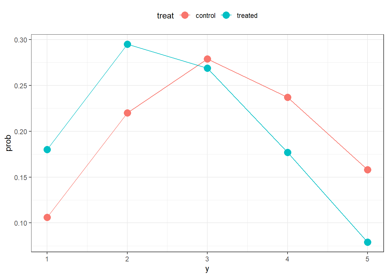
15.1 Now let’s fit a proportion ordinal regression model
Let’s use skeptical prior - normal(0,log(5)/1.96)
# set Priors:
priors <- c(
  set_prior("student_t(3, 0, 5)", class = "Intercept"),  # cutpoints θ1..θ(K-1)
  set_prior("normal(0, 0.8211418)",       class = "b")           # slopes on log-odds
)

#pomod1 <- brm(
#  y ~ treat,                     # add predictors as needed
#  data   = d,
##  family = cumulative("logit"),     # proportional odds
#  prior  = priors,
#  chains = 4, iter = 4000, seed = 123
#)
#let's save the model so we don't have to rerun
#saveRDS(pomod1,file="31_proportional_ord_reg_model_Bayesian_prior0.2-5.0_COR_pomod1.rds")
#read in the model
pomod1<-readRDS(file="31_proportional_ord_reg_model_Bayesian_prior0.2-5.0_COR_pomod1.rds")
summary(pomod1) # get Rhat, ESS
Family: cumulative
Links: mu = logit; disc = identity
Formula: y ~ treat
Data: d (Number of observations: 2000)
Draws: 4 chains, each with iter = 4000; warmup = 2000; thin = 1;
total post-warmup draws = 8000
Regression Coefficients:
Estimate Est.Error l-95% CI u-95% CI Rhat Bulk_ESS Tail_ESS
Intercept[1] -2.20 0.08 -2.36 -2.05 1.00 5095 5221
Intercept[2] -0.89 0.06 -1.01 -0.76 1.00 7354 6821
Intercept[3] 0.39 0.06 0.27 0.51 1.00 8579 7050
Intercept[4] 1.74 0.08 1.59 1.89 1.00 8564 6464
treattreated -0.67 0.08 -0.83 -0.52 1.00 7680 5783
Further Distributional Parameters:
Estimate Est.Error l-95% CI u-95% CI Rhat Bulk_ESS Tail_ESS
disc 1.00 0.00 1.00 1.00 NA NA NA
Draws were sampled using sampling(NUTS). For each parameter, Bulk_ESS
and Tail_ESS are effective sample size measures, and Rhat is the potential
scale reduction factor on split chains (at convergence, Rhat = 1).#plot(pomod1) # trace and densities
pp_check(pomod1,type="bars",ndraws=100) # posterior predictive vs observed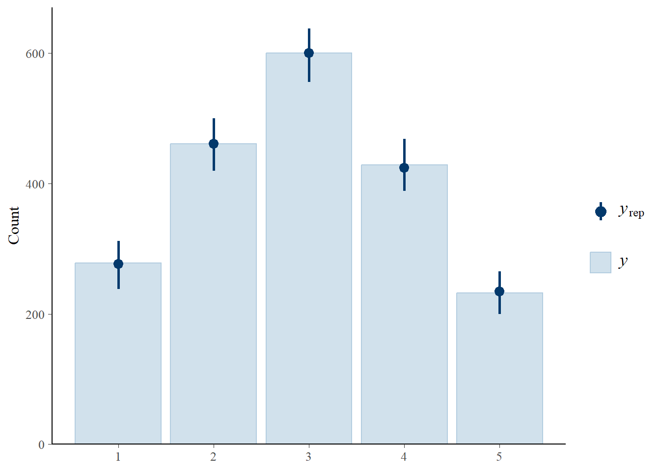
# get model summary - mean and 95% CrI
brms_summary(pomod1)|>
  filter(variable=="b_treattreated")|>
  select(-variable)|>
  exp()
# A tibble: 1 × 4
mean sd `2.5%` `97.5%`
<dbl> <dbl> <dbl> <dbl>
1 0.510 1.09 0.435 0.595#very close to the real estimate, COR = 0.5!
#if close to 1, can test hypotheses about being above or below 1 COR
#chekc proportional odds
# approach - fit with a partial proportional odds model
# here, we suspect that the treatment effect differs by threshold
#then we use leave one out to determine which model is better
#pomod.partial <- brm(
# y ~ cs(treat), # add predictors as needed
# data = d,
# family = cumulative("logit"), # proportional odds
# prior = priors,
# chains = 4, iter = 4000, seed = 123
#)
#save and read in pomod.partial
#saveRDS(pomod.partial,file="31_partial_proportional_ord_reg_model_Bayesian_prior0.2-5.0_COR_pomod.partial.rds")
pomod.partial<-readRDS(file="31_partial_proportional_ord_reg_model_Bayesian_prior0.2-5.0_COR_pomod.partial.rds")
summary(pomod.partial)Warning: Category specific effects for this family should be considered
experimental and may have convergence issues. Family: cumulative
Links: Warning: Category specific effects for this family should be considered
experimental and may have convergence issues.mu = logit; disc = identity
Formula: y ~ cs(treat)
Data: d (Number of observations: 2000)
Draws: 4 chains, each with iter = 4000; warmup = 2000; thin = 1;
total post-warmup draws = 8000
Regression Coefficients:
Estimate Est.Error l-95% CI u-95% CI Rhat Bulk_ESS Tail_ESS
Intercept[1] -2.20 0.10 -2.40 -2.00 1.00 3841 4828
Intercept[2] -0.88 0.07 -1.02 -0.75 1.00 5221 5606
Intercept[3] 0.41 0.06 0.29 0.54 1.00 6711 6156
Intercept[4] 1.72 0.09 1.55 1.90 1.00 6180 6128
treattreated[1] -0.66 0.13 -0.92 -0.41 1.00 4000 4974
treattreated[2] -0.67 0.10 -0.86 -0.48 1.00 5037 5144
treattreated[3] -0.62 0.10 -0.81 -0.43 1.00 5861 5807
treattreated[4] -0.74 0.14 -1.02 -0.46 1.00 6187 6068
Further Distributional Parameters:
Estimate Est.Error l-95% CI u-95% CI Rhat Bulk_ESS Tail_ESS
disc 1.00 0.00 1.00 1.00 NA NA NA
Draws were sampled using sampling(NUTS). For each parameter, Bulk_ESS
and Tail_ESS are effective sample size measures, and Rhat is the potential
scale reduction factor on split chains (at convergence, Rhat = 1).#leave one out analysis
#it is the out-of-sample predictive accuracy
#It asks, which model is better at predicting unseen data?
##output
#elpd_loo → Expected log predictive density
# * higher means better predictive perofrmance , the difference between models matter
#se_elpd_loo → Standard error of elpd
#looic → LOO information criterion (−2 * elpd_loo)
#p_loo → Effective number of parameters
#pareto_k → Diagnostics
#loopo<-loo_compare(loo(pomod1),loo(pomod.partial))
#saveRDS(loopo,file="31_LOO_CMmodels_proportional_2models.rds")
loopo<-readRDS(file="31_LOO_CMmodels_proportional_2models.rds")
knitr::kable(loopo)| elpd_diff | se_diff | elpd_loo | se_elpd_loo | p_loo | se_p_loo | looic | se_looic | |
|---|---|---|---|---|---|---|---|---|
| pomod1 | 0.000000 | 0.000000 | -3076.863 | 16.00865 | 5.030046 | 0.0621834 | 6153.726 | 32.01730 |
| pomod.partial | -2.504103 | 1.009922 | -3079.367 | 16.01258 | 8.021945 | 0.0950263 | 6158.735 | 32.02516 |
pomod1 predicts new data better than pomod.partial (higher ELPD is better; the top row is set to 0 by definition and is the best).
The difference in ELPD is 2.5 with SE = 1.0. A common rule-of-thumb:
if |elpd_diff| > 2 × se_diff, there is strong evidence the top model predicts better.
Here, 2.5/1.0=2.52.5 / 1.0 = 2.52.5/1.0=2.5 ⇒ strong evidence in favor of pomod1.
15.2 Extract predicted probabilities for each category
15.2.1 Not very tidy way of extraction
# predict cateogry probabilities
p_cat <- posterior_epred(pomod1, newdata = tibble(treat=c("control","treated"))) # draws x rows x K
# Posterior means per arm and category:
apply(p_cat, c(2,3), mean) # rows: newdat rows, cols: categories
# 95% CrI:
apply(p_cat, c(2,3), quantile, c(.025,.975))
#not very tidy...15.2.2 Using marginaleffects to extract
This is much cleaner
#set up new data
newd<-tibble(treat=c("control","treated"))
#get marginal probabilities by treatment
avg_pr<-avg_predictions(pomod1,variables="treat",type="response",newdata=newd)
head(avg_pr)
Group treat Estimate 2.5 % 97.5 %
1 control 0.0994 0.086 0.114
1 treated 0.1781 0.157 0.200
2 control 0.1924 0.174 0.212
2 treated 0.2688 0.247 0.291
3 control 0.3039 0.284 0.324
3 treated 0.2958 0.276 0.316
Type: response #let's plot
fig1<-ggplot(avg_pr,aes(y=estimate,x=group,colour=treat,group=treat,fill=treat))+geom_line()+geom_point(size=3)+geom_ribbon(aes(ymin = conf.low,ymax=conf.high),alpha=.1,colour=NA)+theme_bw()+xlab("ordinal scale")+ylab("Probability")+theme(legend.position = "top")
#looks like the original dataset, which is good
#lets get average differences
avg_diff<-avg_comparisons(pomod1,variables="treat")
head(avg_diff)
Group Estimate 2.5 % 97.5 %
1 0.07846 0.0595 0.098338
2 0.07637 0.0583 0.095707
3 -0.00789 -0.0160 -0.000736
4 -0.07970 -0.0997 -0.060925
5 -0.06720 -0.0846 -0.050800
Term: treat
Type: response
Comparison: treated - controlfig2<-avg_diff|>
data.frame()|>
select(-c(term,contrast))|>
ggplot(aes(x=group,y=estimate,group=1))+geom_ribbon(aes(ymin = conf.low,ymax=conf.high),alpha=.1,colour=NA)+geom_point()+geom_line()+theme_bw()+geom_hline(yintercept = 0,lty="dotdash")+xlab("ordinal scale")+ylab("ATE (Treatment-Control)")
(fig1|fig2)+plot_annotation(tag_levels = "A")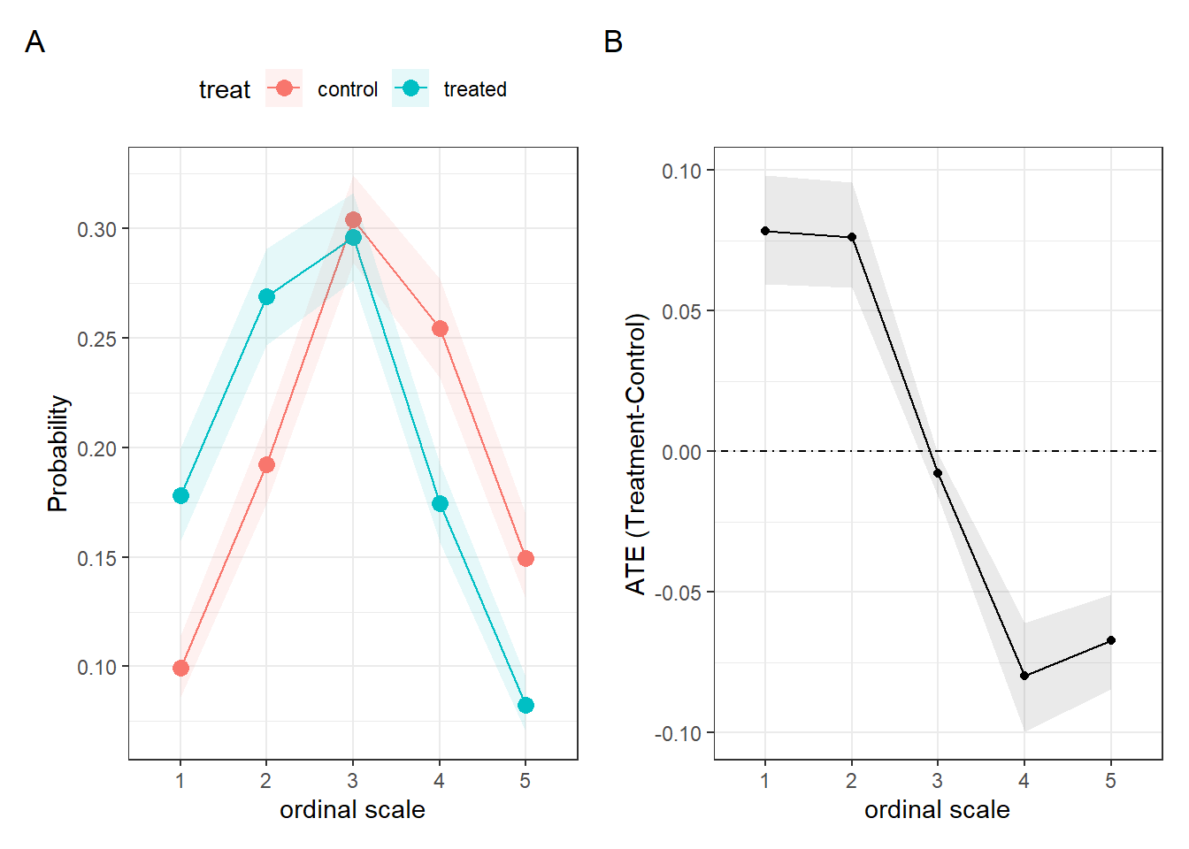
16 Partial proportional ordinal regression model- simulate data first
Let’s say the control mostly die (category 5) compared to treated. So I’ll set the control and treatment to have their own probabilities
#Let's set up probabilities, then add in some simulate outcomes based on those probabilities
ss<-1000 # sample size
control.prob<-c(0.1,.2,.3,.25,.15)
#sum(control.prob)# has to add up to 1
treat.prob<-c(0.025,.025,.025,.025,.9)
#sample data ; control and treatment
#control
control<-sample(size=ss,x=1:5,prob=control.prob,replace=TRUE)
#treatment
trt<-sample(size=ss,x=1:5,prob=treat.prob,replace=TRUE)
#merge dataset
d2<-tibble(y=c(control,trt),treat=c(rep("control",ss),rep("treated",ss)))
head(d2)# A tibble: 6 × 2
y treat
<int> <chr>
1 2 control
2 5 control
3 4 control
4 5 control
5 4 control
6 5 control#levels(factor(d$treat))
#let's plot the data
d2|>
count(treat,y)|>
mutate(prob=n/ss)|>
ggplot(aes(x=y,y=prob,colour=treat))+geom_point(size=4)+geom_line()+theme_bw()+theme(legend.position="top")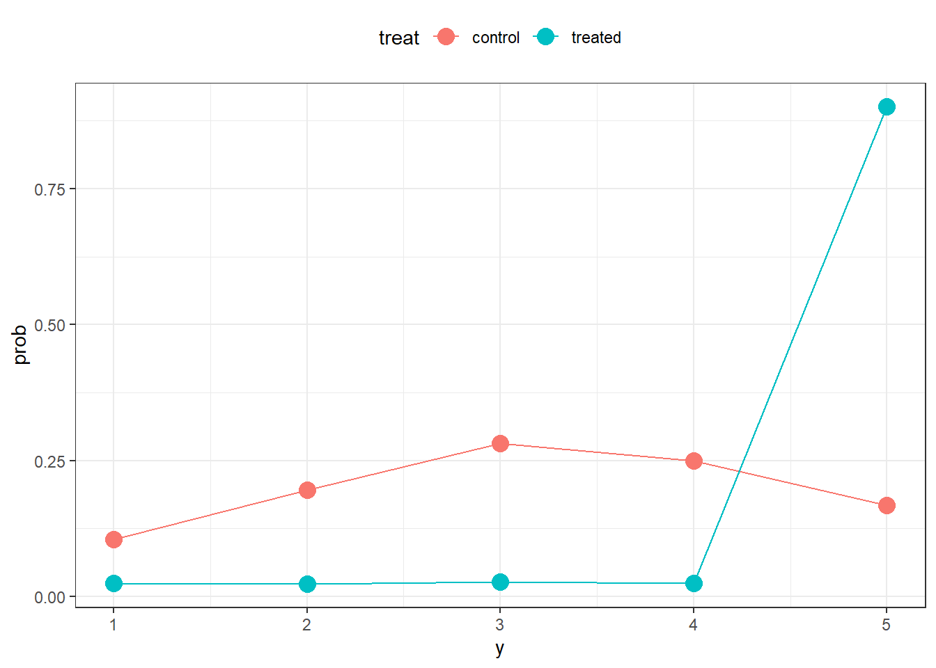
16.1 Fit a partial proportional ordinal regression model
# set Priors:
priors2 <- c(
set_prior("student_t(3, 0, 5)", class = "Intercept"), # cutpoints θ1..θ(K-1)
set_prior("normal(0, 0.8211418)", class = "b") # slopes on log-odds
)
######part.mod1 fit
#part.mod1 <- brm(
# y ~ cs(treat),
# data = d2,
# family = cumulative("logit"),
# prior = priors2,
# chains = 4, iter = 4000, seed = 123
#)
#saveRDS(part.mod1,file="31_part.mod1_bayesian_partialpomod_case_specificfit.rds")
part.mod1<-readRDS(file="31_part.mod1_bayesian_partialpomod_case_specificfit.rds")
summary(part.mod1)Warning: Category specific effects for this family should be considered
experimental and may have convergence issues. Family: cumulative
Links: Warning: Category specific effects for this family should be considered
experimental and may have convergence issues.mu = logit; disc = identity
Formula: y ~ cs(treat)
Data: d2 (Number of observations: 2000)
Draws: 4 chains, each with iter = 4000; warmup = 2000; thin = 1;
total post-warmup draws = 8000
Regression Coefficients:
Estimate Est.Error l-95% CI u-95% CI Rhat Bulk_ESS Tail_ESS
Intercept[1] -2.37 0.11 -2.58 -2.15 1.00 4327 4819
Intercept[2] -0.98 0.07 -1.11 -0.84 1.00 7387 6962
Intercept[3] 0.35 0.06 0.23 0.48 1.00 7596 6966
Intercept[4] 1.66 0.08 1.50 1.82 1.00 6462 6463
treattreated[1] 1.00 0.20 0.61 1.41 1.00 4057 5499
treattreated[2] 1.72 0.14 1.43 2.00 1.00 4101 4716
treattreated[3] 2.68 0.12 2.44 2.92 1.00 4022 4168
treattreated[4] 3.71 0.13 3.46 3.97 1.00 4283 4684
Further Distributional Parameters:
Estimate Est.Error l-95% CI u-95% CI Rhat Bulk_ESS Tail_ESS
disc 1.00 0.00 1.00 1.00 NA NA NA
Draws were sampled using sampling(NUTS). For each parameter, Bulk_ESS
and Tail_ESS are effective sample size measures, and Rhat is the potential
scale reduction factor on split chains (at convergence, Rhat = 1).pp_check(part.mod1,type="bars",ndraws=100) # posterior predictive vs observedWarning: Category specific effects for this family should be considered
experimental and may have convergence issues.
Warning: Category specific effects for this family should be considered
experimental and may have convergence issues.
Warning: Category specific effects for this family should be considered
experimental and may have convergence issues.
Warning: Category specific effects for this family should be considered
experimental and may have convergence issues.
Warning: Category specific effects for this family should be considered
experimental and may have convergence issues.
Warning: Category specific effects for this family should be considered
experimental and may have convergence issues.
Warning: Category specific effects for this family should be considered
experimental and may have convergence issues.
Warning: Category specific effects for this family should be considered
experimental and may have convergence issues.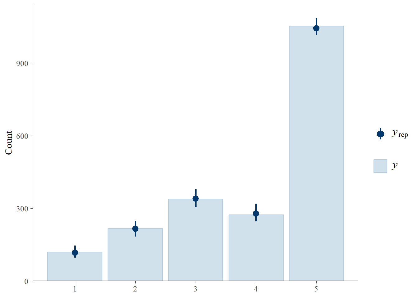
# get model summary - mean and 95% CrI
brms_summary(part.mod1)|>
filter(grepl(variable,pattern="bcs_")==TRUE)|>
mutate(mean=exp(mean),`2.5%`=exp(`2.5%`),`97.5%`=exp(`97.5%`))|>
select(-sd)# A tibble: 4 × 4
variable mean `2.5%` `97.5%`
<chr> <dbl> <dbl> <dbl>
1 bcs_treattreated[1] 2.72 1.84 4.09
2 bcs_treattreated[2] 5.56 4.18 7.37
3 bcs_treattreated[3] 14.5 11.4 18.6
4 bcs_treattreated[4] 40.8 31.9 52.7 conditional_effects(part.mod1,categorical=TRUE)Warning: Category specific effects for this family should be considered
experimental and may have convergence issues.
Warning: Category specific effects for this family should be considered
experimental and may have convergence issues.
Warning: Category specific effects for this family should be considered
experimental and may have convergence issues.
Warning: Category specific effects for this family should be considered
experimental and may have convergence issues.
Warning: Category specific effects for this family should be considered
experimental and may have convergence issues.
Warning: Category specific effects for this family should be considered
experimental and may have convergence issues.
Warning: Category specific effects for this family should be considered
experimental and may have convergence issues.
Warning: Category specific effects for this family should be considered
experimental and may have convergence issues.
Warning: Category specific effects for this family should be considered
experimental and may have convergence issues.
Warning: Category specific effects for this family should be considered
experimental and may have convergence issues.
Warning: Category specific effects for this family should be considered
experimental and may have convergence issues.
Warning: Category specific effects for this family should be considered
experimental and may have convergence issues.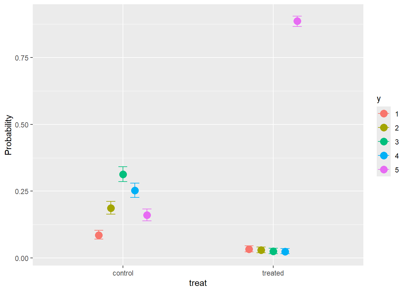
########ACM ordinal regression fit #####################

#the tutorial for ordinal regression in brms recommends different specification:

#case specific effects
#part.mod2 <- brm(
#  y ~ cs(treat),
#  data   = d2,
#  family = acat("probit"),
#  prior  = priors2,
#  chains = 4, iter = 4000, seed = 123
#)
#saveRDS(part.mod2,file="31_part.mod2_bayesian_ACMmod_probit_specificfit.rds")
part.mod2<-readRDS("31_part.mod2_bayesian_ACMmod_probit_specificfit.rds")
summary(part.mod2)
Family: acat
Links: mu = probit; disc = identity
Formula: y ~ cs(treat)
Data: d2 (Number of observations: 2000)
Draws: 4 chains, each with iter = 4000; warmup = 2000; thin = 1;
total post-warmup draws = 8000
Regression Coefficients:
Estimate Est.Error l-95% CI u-95% CI Rhat Bulk_ESS Tail_ESS
Intercept[1] -0.46 0.08 -0.62 -0.31 1.00 6918 6328
Intercept[2] -0.31 0.06 -0.43 -0.20 1.00 6043 5701
Intercept[3] 0.15 0.05 0.05 0.26 1.00 5715 5762
Intercept[4] 0.29 0.06 0.17 0.42 1.00 6162 6098
treattreated[1] -0.52 0.18 -0.87 -0.16 1.00 6062 5952
treattreated[2] -0.38 0.18 -0.74 -0.04 1.00 5296 5135
treattreated[3] 0.17 0.18 -0.18 0.53 1.00 5832 5618
treattreated[4] 2.24 0.10 2.04 2.44 1.00 5220 5612
Further Distributional Parameters:
Estimate Est.Error l-95% CI u-95% CI Rhat Bulk_ESS Tail_ESS
disc 1.00 0.00 1.00 1.00 NA NA NA
Draws were sampled using sampling(NUTS). For each parameter, Bulk_ESS
and Tail_ESS are effective sample size measures, and Rhat is the potential
scale reduction factor on split chains (at convergence, Rhat = 1).conditional_effects(part.mod2,categorical=TRUE)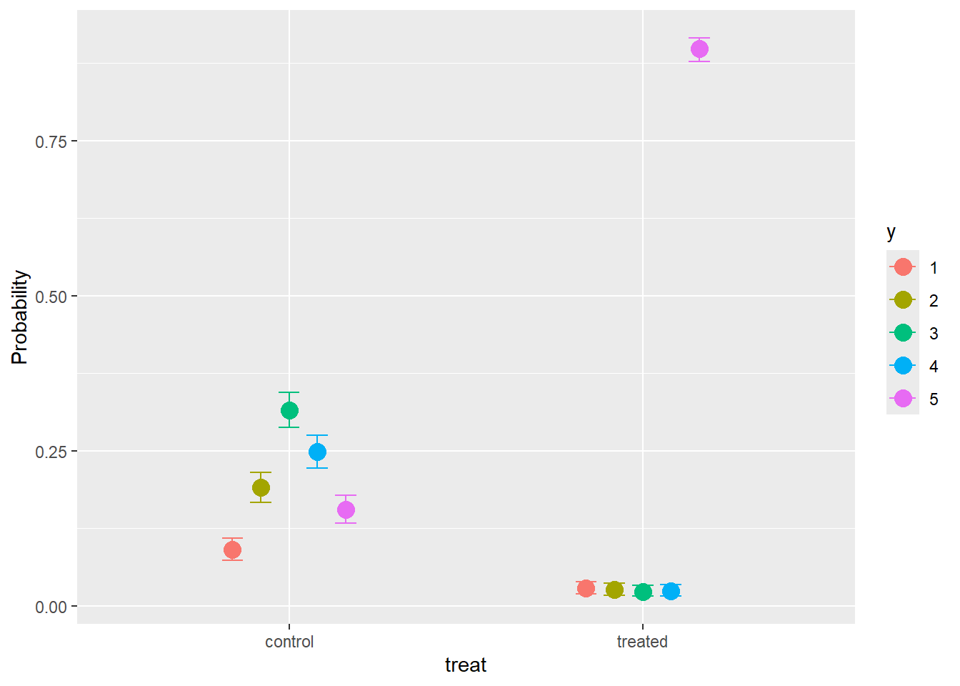
#proportional effects
#part.mod3 <- brm(
#  y ~ treat,
#  data   = d2,
#  family = acat("probit"),
#  prior  = priors2,
#  chains = 4, iter = 4000, seed = 123
#)
#saveRDS(part.mod3,file="31_part.mod3_bayesian_ACMmod_probit_NO_specificfit.rds")
part.mod3<-readRDS("31_part.mod3_bayesian_ACMmod_probit_NO_specificfit.rds")
summary(part.mod3)
Family: acat
Links: mu = probit; disc = identity
Formula: y ~ treat
Data: d2 (Number of observations: 2000)
Draws: 4 chains, each with iter = 4000; warmup = 2000; thin = 1;
total post-warmup draws = 8000
Regression Coefficients:
Estimate Est.Error l-95% CI u-95% CI Rhat Bulk_ESS Tail_ESS
Intercept[1] -0.33 0.07 -0.46 -0.20 1.00 7203 6175
Intercept[2] -0.18 0.05 -0.29 -0.08 1.00 6743 6401
Intercept[3] 0.40 0.05 0.30 0.50 1.00 5551 5340
Intercept[4] -0.33 0.05 -0.42 -0.23 1.00 4602 5067
treattreated 0.84 0.04 0.77 0.91 1.00 5488 5533
Further Distributional Parameters:
Estimate Est.Error l-95% CI u-95% CI Rhat Bulk_ESS Tail_ESS
disc 1.00 0.00 1.00 1.00 NA NA NA
Draws were sampled using sampling(NUTS). For each parameter, Bulk_ESS
and Tail_ESS are effective sample size measures, and Rhat is the potential
scale reduction factor on split chains (at convergence, Rhat = 1).conditional_effects(part.mod3,categorical=TRUE)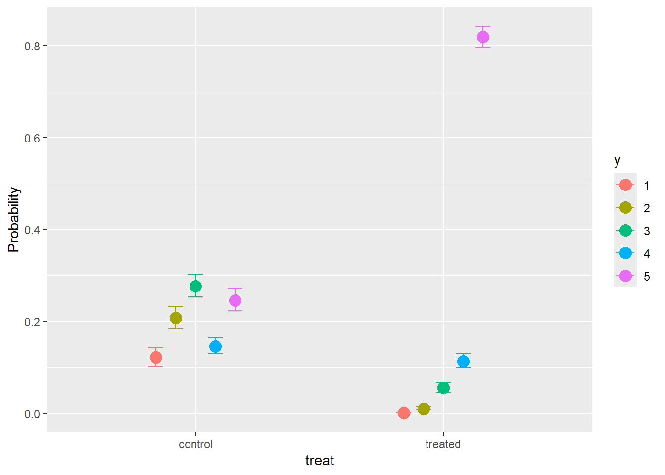
#######

###now comparing with proportional ordinal regression model
#Leave one out cross validation
#In the context of model selection, a LOO difference greater than twice its corresponding
#standard error can be interpreted as suggesting that the model with a lower LOO value fits
#the data substantially better, at least when the number of observations is large enough
#loopartial<-loo_compare(loo(part.mod1),loo(part.mod2),loo(part.mod3))
#saveRDS(loopartial,file="31_LOO_partial_proportional_3models.rds")
loopartial<-readRDS(file="31_LOO_partial_proportional_3models.rds")
knitr::kable(loopartial)| elpd_diff | se_diff | elpd_loo | se_elpd_loo | p_loo | se_p_loo | looic | se_looic | |
|---|---|---|---|---|---|---|---|---|
| part.mod2 | 0.000000 | 0.000000 | -2005.378 | 43.31267 | 7.742633 | 0.3534608 | 4010.757 | 86.62534 |
| part.mod1 | -1.114306 | 1.511076 | -2006.493 | 42.47984 | 7.677652 | 0.3580129 | 4012.985 | 84.95968 |
| part.mod3 | -195.829880 | 21.704605 | -2201.208 | 48.65666 | 6.295668 | 0.3558727 | 4402.417 | 97.31331 |
The case specific effects models are more favorable models. Out of the case specific effects models, specifying with the model is ACM (acat) or CM yield similar models.
17 Now, analyzing a continuous variable with ordinal regression
co<-rnorm(n=ss,50,5)
t<-co+rnorm(n=ss,5,1)
cond<-tibble(y=c(co,t),treat=c(rep("control",ss),rep("treated",ss)))
ggplot(cond,aes(y=treat,x=y,fill=treat))+stat_halfeye() 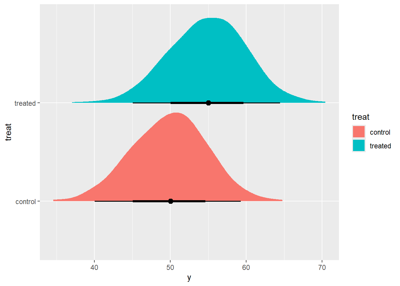
#let's convert to ordinal scale
cond$yord<-factor(round(cond$y,0),ordered=TRUE)

##set up prior
priors3 <- c(
  set_prior("student_t(3, 0, 5)", class = "Intercept"),  # cutpoints θ1..θ(K-1)
  set_prior("normal(0, 2.349577)",       class = "b")           # slopes on log-odds
)
# I don't know what is plausible for cumulative odds ratio -> so I'll use a diffuse prior log(100)/1.96

#let's fit proportional CM model
#comod1 <- brm(
#  yord ~ treat,
#  data   = cond,
#  family = cumulative("logit"),     # proportional odds
# prior  = priors3,
#  chains = 4, iter = 4000, seed = 123,control = list(adapt_delta = 0.98)
#)
#saveRDS(comod1,file="31_comod1_ord_reg_CMmod_continuous_outcome_converted_to_ordinal.rds")
comod1<-readRDS(file="31_comod1_ord_reg_CMmod_continuous_outcome_converted_to_ordinal.rds")
summary(comod1) # get Rhat, ESS
Family: cumulative
Links: mu = logit; disc = identity
Formula: yord ~ treat
Data: cond (Number of observations: 2000)
Draws: 4 chains, each with iter = 4000; warmup = 2000; thin = 1;
total post-warmup draws = 8000
Regression Coefficients:
Estimate Est.Error l-95% CI u-95% CI Rhat Bulk_ESS Tail_ESS
Intercept[1] -8.17 1.20 -11.06 -6.30 1.00 5598 3815
Intercept[2] -6.91 0.75 -8.60 -5.63 1.00 8848 5971
Intercept[3] -6.22 0.57 -7.44 -5.22 1.00 10547 5967
Intercept[4] -5.41 0.41 -6.27 -4.69 1.00 10932 6411
Intercept[5] -4.92 0.33 -5.61 -4.32 1.00 10855 6167
Intercept[6] -4.20 0.23 -4.68 -3.77 1.00 11821 6442
Intercept[7] -3.58 0.17 -3.93 -3.25 1.00 15388 5907
Intercept[8] -3.31 0.15 -3.62 -3.02 1.00 14351 6589
Intercept[9] -2.95 0.13 -3.21 -2.70 1.00 13103 6443
Intercept[10] -2.46 0.11 -2.67 -2.25 1.00 13054 6975
Intercept[11] -1.98 0.09 -2.16 -1.81 1.00 11912 6538
Intercept[12] -1.56 0.08 -1.71 -1.41 1.00 12340 7074
Intercept[13] -1.16 0.07 -1.29 -1.02 1.00 11755 7231
Intercept[14] -0.80 0.06 -0.93 -0.68 1.00 12043 6939
Intercept[15] -0.50 0.06 -0.62 -0.38 1.00 11957 7366
Intercept[16] -0.21 0.06 -0.33 -0.09 1.00 10410 7020
Intercept[17] 0.19 0.06 0.07 0.31 1.00 10109 6860
Intercept[18] 0.48 0.06 0.36 0.60 1.00 10274 5944
Intercept[19] 0.80 0.06 0.68 0.93 1.00 9636 6098
Intercept[20] 1.16 0.07 1.03 1.29 1.00 9968 6741
Intercept[21] 1.45 0.07 1.32 1.59 1.00 10270 5867
Intercept[22] 1.79 0.07 1.65 1.94 1.00 10347 5707
Intercept[23] 2.04 0.08 1.90 2.19 1.00 10240 6232
Intercept[24] 2.41 0.08 2.26 2.57 1.00 10380 5598
Intercept[25] 2.71 0.08 2.55 2.88 1.00 9932 5925
Intercept[26] 3.07 0.09 2.90 3.25 1.00 11395 6101
Intercept[27] 3.43 0.10 3.24 3.62 1.00 10958 5636
Intercept[28] 3.74 0.11 3.53 3.95 1.00 12158 6322
Intercept[29] 4.13 0.12 3.89 4.37 1.00 12071 5598
Intercept[30] 4.74 0.15 4.45 5.04 1.00 13188 6087
Intercept[31] 5.39 0.19 5.02 5.79 1.00 12458 6275
Intercept[32] 6.18 0.28 5.66 6.77 1.00 14824 5474
Intercept[33] 6.58 0.33 5.97 7.26 1.00 14198 6176
Intercept[34] 7.61 0.51 6.69 8.70 1.00 13512 4656
Intercept[35] 9.42 1.14 7.64 12.15 1.00 11618 5545
treattreated 1.72 0.08 1.56 1.88 1.00 9282 5567
Further Distributional Parameters:
Estimate Est.Error l-95% CI u-95% CI Rhat Bulk_ESS Tail_ESS
disc 1.00 0.00 1.00 1.00 NA NA NA
Draws were sampled using sampling(NUTS). For each parameter, Bulk_ESS
and Tail_ESS are effective sample size measures, and Rhat is the potential
scale reduction factor on split chains (at convergence, Rhat = 1).#plot(comod1)
pp_check(comod1,type="bars",ndraws=100) # posterior predictive vs observed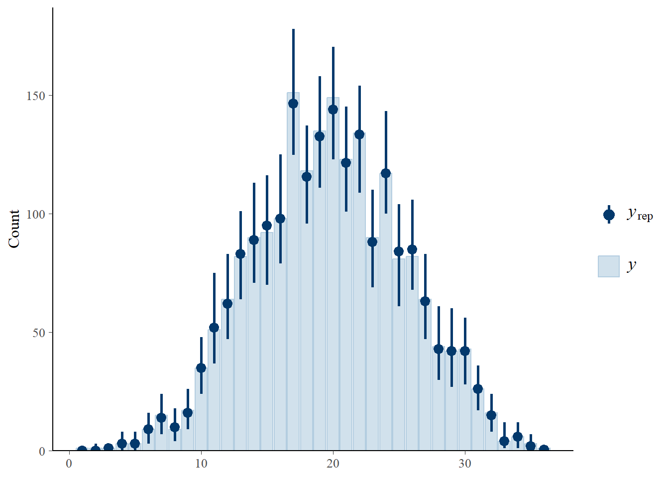
# get model summary - mean and 95% CrI
brms_summary(comod1)|>
  filter(variable=="b_treattreated")|>
  select(-variable)|>
  exp()
# A tibble: 1 × 4
mean sd `2.5%` `97.5%`
<dbl> <dbl> <dbl> <dbl>
1 5.58 1.09 4.74 6.56# The cumulative odds is 5.58 and this means that the treated increases the odds by 5.58 to being in a higher ranked category.
conditional_effects(comod1,categorical=TRUE)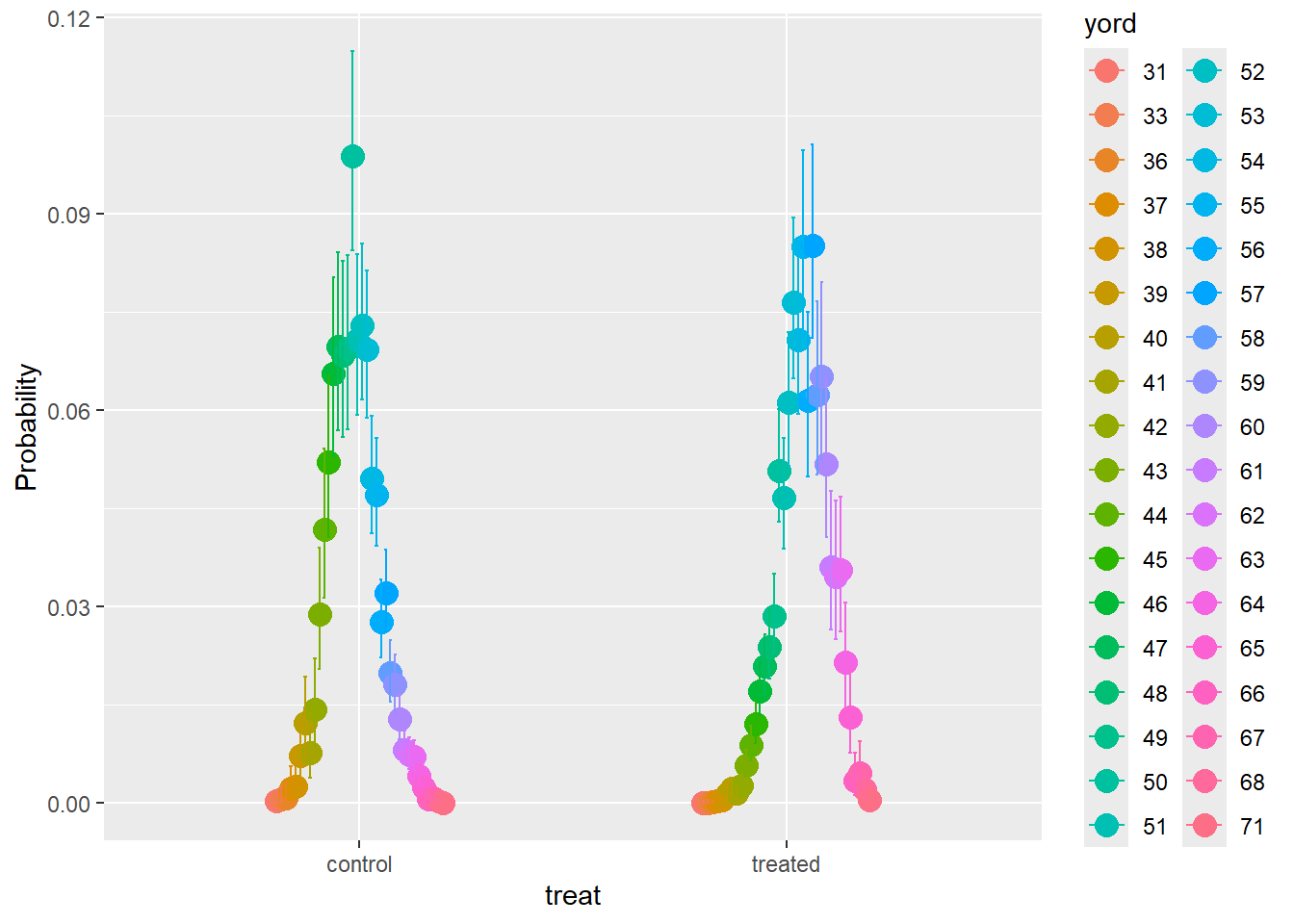
#how many levels do i ahve?
length(levels(comod1$data$yord))
[1] 36Notes- ordinal regression can work on continuous data, which means that you can break a continuous scale into ordinal values. This may be important for cases where you want to merge a continuous outcome with a terminal, absorbing state (death). In our case, 71 was highest continuous scale, and if we wanted to include death, then 72 could be representing death.
To better obtain convergence of chains, the adapt_delta was set to 0.98. At adapt_delta set to 0.95, there were divergent chains.
18 Session info
sessionInfo()R version 4.5.0 (2025-04-11 ucrt)
Platform: x86_64-w64-mingw32/x64
Running under: Windows 11 x64 (build 26100)
Matrix products: default
LAPACK version 3.12.1
locale:
[1] LC_COLLATE=English_United States.utf8
[2] LC_CTYPE=English_United States.utf8
[3] LC_MONETARY=English_United States.utf8
[4] LC_NUMERIC=C
[5] LC_TIME=English_United States.utf8
time zone: America/New_York
tzcode source: internal
attached base packages:
[1] splines stats graphics grDevices utils datasets methods
[8] base
other attached packages:
[1] tidybayes_3.0.7 patchwork_1.3.0 ggbeeswarm_0.7.2
[4] marginaleffects_0.25.1 brms_2.22.0 Rcpp_1.0.14
[7] gt_1.0.0 gtsummary_2.2.0 lubridate_1.9.4
[10] forcats_1.0.0 stringr_1.5.1 dplyr_1.1.4
[13] purrr_1.0.4 readr_2.1.5 tidyr_1.3.1
[16] tibble_3.2.1 ggplot2_3.5.2 tidyverse_2.0.0
loaded via a namespace (and not attached):
[1] tidyselect_1.2.1 svUnit_1.0.6 vipor_0.4.7
[4] farver_2.1.2 loo_2.8.0 fastmap_1.2.0
[7] tensorA_0.36.2.1 digest_0.6.37 timechange_0.3.0
[10] lifecycle_1.0.4 StanHeaders_2.32.10 magrittr_2.0.3
[13] posterior_1.6.1 compiler_4.5.0 rlang_1.1.6
[16] tools_4.5.0 utf8_1.2.4 yaml_2.3.10
[19] collapse_2.1.6 data.table_1.17.0 knitr_1.50
[22] labeling_0.4.3 bridgesampling_1.1-2 htmlwidgets_1.6.4
[25] pkgbuild_1.4.7 curl_6.2.2 plyr_1.8.9
[28] xml2_1.3.8 abind_1.4-8 withr_3.0.2
[31] grid_4.5.0 stats4_4.5.0 colorspace_2.1-1
[34] inline_0.3.21 scales_1.3.0 insight_1.1.0
[37] cli_3.6.4 mvtnorm_1.3-3 rmarkdown_2.29
[40] generics_0.1.3 RcppParallel_5.1.10 reshape2_1.4.4
[43] tzdb_0.5.0 rstan_2.32.7 bayesplot_1.12.0
[46] parallel_4.5.0 matrixStats_1.5.0 vctrs_0.6.5
[49] V8_6.0.3 Matrix_1.7-3 jsonlite_2.0.0
[52] hms_1.1.3 arrayhelpers_1.1-0 beeswarm_0.4.0
[55] ggdist_3.3.2 glue_1.8.0 codetools_0.2-20
[58] distributional_0.5.0 stringi_1.8.7 gtable_0.3.6
[61] QuickJSR_1.7.0 munsell_0.5.1 pillar_1.10.2
[64] htmltools_0.5.8.1 Brobdingnag_1.2-9 R6_2.6.1
[67] evaluate_1.0.3 lattice_0.22-6 backports_1.5.0
[70] rstantools_2.4.0 coda_0.19-4.1 gridExtra_2.3
[73] nlme_3.1-168 checkmate_2.3.2 xfun_0.52
[76] pkgconfig_2.0.3