library(tidyverse) # for ggplot2, data visualization and data filtering with dplyr
library(ggbeeswarm) # for quasirandom plotting
library(pwr) # power analysis
library(gsDesign) # power analysis for survival
library(blockrand) # randomization package
library(randomizeR)# another randomization package

#ggplot2 settings I like:
T<-theme_bw()+theme(,text=element_text(size=18),
                    axis.text=element_text(size=18),
                    panel.grid.major=element_blank(),
                    panel.grid.minor.x = element_blank(),
                    panel.grid = element_blank(),
                    legend.key = element_blank(),
                    axis.title.y=element_text(margin=margin(t=0,r=15,b=0,l=0)),
                    axis.title.x=element_text(margin=margin(t=15,r=,b=0,l=0)))
#+ theme(legend.position="none")14 Randomization and sample size estimation
15 Introduction:
The aim of this demo is to showcase how to estimate sample sizes and conduct randomization in clinical trial designs. R has a suite of packages geared towards clinical trial design, monitoring, and analyses (CRAN R Projects- Clinical Trials Zhang, Zhang, and Zhang (2021)). I’m also modeling my demo off of Peter Higgin’s Reproducible Medical Research with R book, chapter 20 (Higgins (2023)).
16 Load Libraries
17 Sample size calculations
It is important to find the appropriate number of participants in a clinical trial because too few participants may lead to an inability to detect differences (studies may be underpowered) and too many participants lead to excessive use of resources.
The critical information to obtain are:
- alpha (\(\alpha\)) level - probability of committing a type I error (false positive)
- beta (\(\beta\)) level - probability of committing a type II error (false negative)
- sometimes the program will ask for power, which is 1-\(\beta\) and is the probability of detecting differences if they truly exist
- sometimes the program will ask for power, which is 1-\(\beta\) and is the probability of detecting differences if they truly exist
- effect size between groups (cohen’s d)
- Note that cohen’s d is expressed as: \(\frac{(\bar\mu_1 - \bar\mu_2)}{S_{pooled}}\), where \(\bar\mu_1\) is the mean of one group and \(\bar\mu_2\) is the mean of the other group, and \(S_{pooled}\) is the pooled standard deviation. Therefore, cohen’s d is interpreted in units of standard deviation.
- Note that cohen’s d is expressed as: \(\frac{(\bar\mu_1 - \bar\mu_2)}{S_{pooled}}\), where \(\bar\mu_1\) is the mean of one group and \(\bar\mu_2\) is the mean of the other group, and \(S_{pooled}\) is the pooled standard deviation. Therefore, cohen’s d is interpreted in units of standard deviation.
- drop out rates
Other information to consider for survival analyses:
- rate of enrollment
- length of study
- hazard rate of each group
17.1 T-test designs and sample size calculations
We will be using the pwr package. To start, let’s estimate a sample size with:
- alpha = 0.05
- power = 0.80 (1-\(\beta\))
- effect size, cohen’s d = 0.5, which is considered a moderate effect size
pwr::pwr.t.test(sig.level=0.05,type="two.sample",power=.8,d=.5)
     Two-sample t test power calculation

              n = 63.76561
              d = 0.5
      sig.level = 0.05
          power = 0.8
    alternative = two.sided

NOTE: n is number in *each* group
Key result: 64 volunteers per arm. We round up because there can be no fractional individuals.
For a different study design, let’s assume there is a before and after measurement of a continuous variable and this would produce paired results with the same assumptions about \(\alpha\),\(\beta\), and cohen’s d.
pwr::pwr.t.test(sig.level=0.05,type="paired",power=.8,d=.5)
     Paired t test power calculation

              n = 33.36713
              d = 0.5
      sig.level = 0.05
          power = 0.8
    alternative = two.sided

NOTE: n is number of *pairs*
Key result: 34 volunteers per arm.
We also may need to consider drop out rates. For example, if there is a 20% drop out rate, then add 20% to the sample sizes per arm. 34 x 20% = ~7, so we would need 41 volunteers.
17.1.1 Simulating effect sizes and power
What if we don’t know the effect size and want to find out sample sizes based on different inputs of effect size and power?
- simulating effect sizes from 0 to 2 in .1 increments
- over two levels of power (0.8 and .9)
#code to get sample size from pwr.t.test
#round(pwr::pwr.t.test(sig.level=0.05,type="two.sample",power=.8,d=c(.5),n=NULL)$n,0)

d<-data.frame(efsize=rep(seq(0.1,2,.1),2),
              power=c(rep(.8,length(seq(0.1,2,.1))),
                      rep(.9,length(seq(0.1,2,.1)))))
d%>%
  group_by(efsize,power)%>%
  mutate(n=round(pwr::pwr.t.test(sig.level=0.05,
                                 type="two.sample",power=power,
                                 d=efsize,n=NULL)$n,0),
         power2=paste("Power = ",power,sep=""))%>%
  #power2 is for plotting
  ggplot(.,aes(x=efsize,y=n,colour=factor(power)))+
  geom_point()+geom_line()+
  theme_minimal()+
  geom_text(aes(label=n),vjust=-1)+
  facet_wrap(~power2,ncol=1)+
  xlab("Effect size (cohen's d)")+
  ylab("Sample size per arm")+
  theme(legend.position = "none")+
  scale_x_continuous(,limits=c(0,2)
                     ,breaks=seq(0,2,.25),
                     labels=seq(0,2,.25))+
  scale_y_continuous(limits=c(0,2500))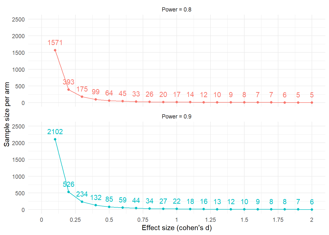
17.2 Chi-square 2x2 contingency table design
In this design, let’s say there are counts of diseased and not-diseased individuals that were exposed and not exposed to some chemical. We want to find the association between the two variables and we need to specify the expected proportions of the 2x2 under the alternative hypothesis.
#ES.w2() # chi-square for test of association
#pwr.chisq.test()

d2<-data.frame(exposure=c("exposed","not exposed"),non_diseased=c(.25,.3),diseased=c(0.25,.2))
knitr::kable(d2)| exposure | non_diseased | diseased |
|---|---|---|
| exposed | 0.25 | 0.25 |
| not exposed | 0.30 | 0.20 |
Now that we have the expected 2x2 matrix under the alternative hypothesis (not independent), then we need to identify the effect size with ES.w2() and then plug and chug with pwr.chisq.test() with \(\alpha\) = 0.05 and power = 0.8.
ef.sim.dat<-ES.w2(d2[,-1])
pwr.chisq.test(w=ef.sim.dat,df=1,power=.8,sig.level=.05)
     Chi squared power calculation

              w = 0.1005038
              N = 777.0372
             df = 1
      sig.level = 0.05
          power = 0.8

NOTE: N is the number of observations
Key result: We need 778 observations. Note that the degrees of freedom on 1 in this case for a 2x2 contingency table, which is calculated as (# of columns - 1) x (# of rows -1).
17.3 Time to event types of designs (survival analyses)
I will be using the gsDesign package and referencing an online resource here.
hr=.7 # hazard ratio
controlMedian<-8 # 8 months
lambda1 <- log(2) / controlMedian #estimated hazard rate of control

nSurvival(
  lambda1 = lambda1,
  lambda2 = lambda1 * hr, #hazard rate for experimental
  Ts = 24, #24 months
  Tr = 6, # 6 months
  eta = .1, # value per month dropout rate
  ratio = 1, # equal sampling
  alpha = .05,
  beta = .2
)
Fixed design, two-arm trial with time-to-event
outcome (Lachin and Foulkes, 1986).
Study duration (fixed): Ts=24
Accrual duration (fixed): Tr=6
Uniform accrual: entry="unif"
Control median: log(2)/lambda1=8
Experimental median: log(2)/lambda2=11.4
Censoring median: log(2)/eta=6.9
Control failure rate: lambda1=0.087
Experimental failure rate: lambda2=0.061
Censoring rate: eta=0.1
Power: 100*(1-beta)=80%
Type I error (1-sided): 100*alpha=5%
Equal randomization: ratio=1
Sample size based on hazard ratio=0.7 (type="rr")
Sample size (computed): n=476
Events required (computed): nEvents=19518 Randomization (stratified permuted block randomization)
Using the t-test design (2 trial arms), we’d like to implement block randomization across a strata. Often times, we can’t sample participants all at once and so we need to apply treatments in groupings as they enroll in the study, or blocks. To ensure equal sampling of treatments across different sub-populations, randomization can be conducted at the level of different sub-populations (strata). For example, randomization can be conducted for males and females separately. With a sample size of 200 per arm, in a two-arm trial, I’m randomization across a gender strata (100 each so they’re equally sampled).
18.1 …with blockrand package
mrand<-blockrand(n = 100,
                     num.levels = 2, # three treatments
                     levels = c("Con.Arm", "Treat.Arm"), # arm names
                     stratum = "Strat.male", # stratum name
                     id.prefix = "SM", # stratum abbrev
                     block.sizes = c(3,4), # times arms = 6,8
                     block.prefix = "blksm") # stratum abbrev

frand<-blockrand(n = 100,
                     num.levels = 2, # three treatments
                     levels = c("Con.Arm", "Treat.Arm"), # arm names
                     stratum = "Strat.female", # stratum name
                     id.prefix = "SF", # stratum abbrev
                     block.sizes = c(3,4), # times arms = 6,8
                     block.prefix = "blkfm") # stratum abbrev
totrand<-rbind(mrand,frand)
knitr::kable(head(totrand,25))| id | stratum | block.id | block.size | treatment |
|---|---|---|---|---|
| SM001 | Strat.male | blksm01 | 6 | Treat.Arm |
| SM002 | Strat.male | blksm01 | 6 | Con.Arm |
| SM003 | Strat.male | blksm01 | 6 | Treat.Arm |
| SM004 | Strat.male | blksm01 | 6 | Treat.Arm |
| SM005 | Strat.male | blksm01 | 6 | Con.Arm |
| SM006 | Strat.male | blksm01 | 6 | Con.Arm |
| SM007 | Strat.male | blksm02 | 6 | Treat.Arm |
| SM008 | Strat.male | blksm02 | 6 | Treat.Arm |
| SM009 | Strat.male | blksm02 | 6 | Con.Arm |
| SM010 | Strat.male | blksm02 | 6 | Con.Arm |
| SM011 | Strat.male | blksm02 | 6 | Con.Arm |
| SM012 | Strat.male | blksm02 | 6 | Treat.Arm |
| SM013 | Strat.male | blksm03 | 8 | Treat.Arm |
| SM014 | Strat.male | blksm03 | 8 | Con.Arm |
| SM015 | Strat.male | blksm03 | 8 | Con.Arm |
| SM016 | Strat.male | blksm03 | 8 | Con.Arm |
| SM017 | Strat.male | blksm03 | 8 | Treat.Arm |
| SM018 | Strat.male | blksm03 | 8 | Treat.Arm |
| SM019 | Strat.male | blksm03 | 8 | Treat.Arm |
| SM020 | Strat.male | blksm03 | 8 | Con.Arm |
| SM021 | Strat.male | blksm04 | 6 | Con.Arm |
| SM022 | Strat.male | blksm04 | 6 | Con.Arm |
| SM023 | Strat.male | blksm04 | 6 | Con.Arm |
| SM024 | Strat.male | blksm04 | 6 | Treat.Arm |
| SM025 | Strat.male | blksm04 | 6 | Treat.Arm |
We can then create patient randomization “cards” based on the blockrand() output.
plotblockrand(totrand,'mystudy.pdf',
              top=list(text=c('MyStudy','Patient:%ID%','Treatment:%TREAT%'),
                       col=c('black','black','red'),font=c(1,1,4)),
              middle=list(text=c("MyStudy","Sex:%STRAT%","Patient:%ID%"),
                          col=c('black','blue','green'),font=c(1,2,3)),
              bottom="Call123-4567toreportpatiententry", cut.marks=TRUE)
18.2 …with randomizeR package
Using the randomized permuted block randomization function, rpbrPar(). The details:
Fix the possible random block lengths rb, the number of treatment groups K, the sample size N and the vector of the ratio. Afterwards, one block length is randomly selected of the random block lengths. The patients are assigned according to the ratio to the corresponding treatment groups. This procedure is repeated until N patients are assigned. Within each block all possible randomization sequences are equiprobable.
#randomization parameters
males<-rpbrPar(N=100, #total sample size
               rb=6, # block length parameter
               K=2) # number of groups
rr<-genSeq(males) # saving randomization procedure
rr.out<-as.vector(getRandList(rr))# grab randomizations
#put into dataframe and make it look better
male.r.dat<-data.frame(sex="M",
                       subject=paste("SM",
                                     seq(1:length(rr.out)),sep=""),
                       treatment=rr.out,
                       treatmentname=ifelse(rr.out=="A","Control","Treatment"))
#male.r.dat
knitr::kable(head(male.r.dat,10))| sex | subject | treatment | treatmentname |
|---|---|---|---|
| M | SM1 | A | Control |
| M | SM2 | B | Treatment |
| M | SM3 | A | Control |
| M | SM4 | A | Control |
| M | SM5 | B | Treatment |
| M | SM6 | B | Treatment |
| M | SM7 | A | Control |
| M | SM8 | A | Control |
| M | SM9 | B | Treatment |
| M | SM10 | B | Treatment |
19 Session Info
sessionInfo()R version 4.5.0 (2025-04-11 ucrt)
Platform: x86_64-w64-mingw32/x64
Running under: Windows 11 x64 (build 26100)
Matrix products: default
LAPACK version 3.12.1
locale:
[1] LC_COLLATE=English_United States.utf8
[2] LC_CTYPE=English_United States.utf8
[3] LC_MONETARY=English_United States.utf8
[4] LC_NUMERIC=C
[5] LC_TIME=English_United States.utf8
time zone: America/New_York
tzcode source: internal
attached base packages:
[1] stats graphics grDevices utils datasets methods base
other attached packages:
[1] randomizeR_3.0.2 mvtnorm_1.3-3 survival_3.8-3 plotrix_3.8-4
[5] blockrand_1.5 gsDesign_3.6.7 pwr_1.3-0 ggbeeswarm_0.7.2
[9] lubridate_1.9.4 forcats_1.0.0 stringr_1.5.1 dplyr_1.1.4
[13] purrr_1.0.4 readr_2.1.5 tidyr_1.3.1 tibble_3.2.1
[17] ggplot2_3.5.2 tidyverse_2.0.0
loaded via a namespace (and not attached):
[1] gtable_0.3.6 beeswarm_0.4.0 xfun_0.52 coin_1.4-3
[5] htmlwidgets_1.6.4 insight_1.1.0 lattice_0.22-6 tzdb_0.5.0
[9] vctrs_0.6.5 tools_4.5.0 generics_0.1.3 sandwich_3.1-1
[13] stats4_4.5.0 parallel_4.5.0 pkgconfig_2.0.3 Matrix_1.7-3
[17] gt_1.0.0 lifecycle_1.0.4 farver_2.1.2 compiler_4.5.0
[21] munsell_0.5.1 codetools_0.2-20 PwrGSD_2.3.8 vipor_0.4.7
[25] htmltools_0.5.8.1 yaml_2.3.10 pillar_1.10.2 MASS_7.3-65
[29] multcomp_1.4-28 r2rtf_1.1.4 tidyselect_1.2.1 digest_0.6.37
[33] stringi_1.8.7 reshape2_1.4.4 labeling_0.4.3 splines_4.5.0
[37] fastmap_1.2.0 grid_4.5.0 colorspace_2.1-1 cli_3.6.4
[41] magrittr_2.0.3 TH.data_1.1-3 libcoin_1.0-10 withr_3.0.2
[45] scales_1.3.0 timechange_0.3.0 rmarkdown_2.29 matrixStats_1.5.0
[49] zoo_1.8-14 modeltools_0.2-23 hms_1.1.3 evaluate_1.0.3
[53] knitr_1.50 rlang_1.1.6 Rcpp_1.0.14 xtable_1.8-4
[57] glue_1.8.0 xml2_1.3.8 jsonlite_2.0.0 R6_2.6.1
[61] plyr_1.8.9